In this vignette, we implement simulation for a dose-ranging trial under adaptive design. We start from a placebo arm and a treatment arm with highest possible dose. At an interim, if we observe promising results, we add arms with doses in between to inform decision at final analysis.
For the sake of simplicity, we assume a binary endpoint of interest.
The response rates at doses 0 (placebo), 0.5, 1.5, 2.5, 4 (highest dose)
are given by a sigEmax model below, where the response rate
is assume to be 10% in placebo, and 25% in arm of the highest dose (dose
= 4). For further background information, refer to vignette
of the DoseFinding package.
mods <- DoseFinding::Mods(sigEmax = rbind(c(1, 3)),
                          placEff = log(.1/(1 - .1)),
                          maxEff = log(.25/(1 - .25)) - log(.1/(1 - .1)),
                          doses = c(0, 0.5, 1.5, 2.5, 4))

DoseFinding::plotMods(mods, trafo = function(x) 1/(1+exp(-x)))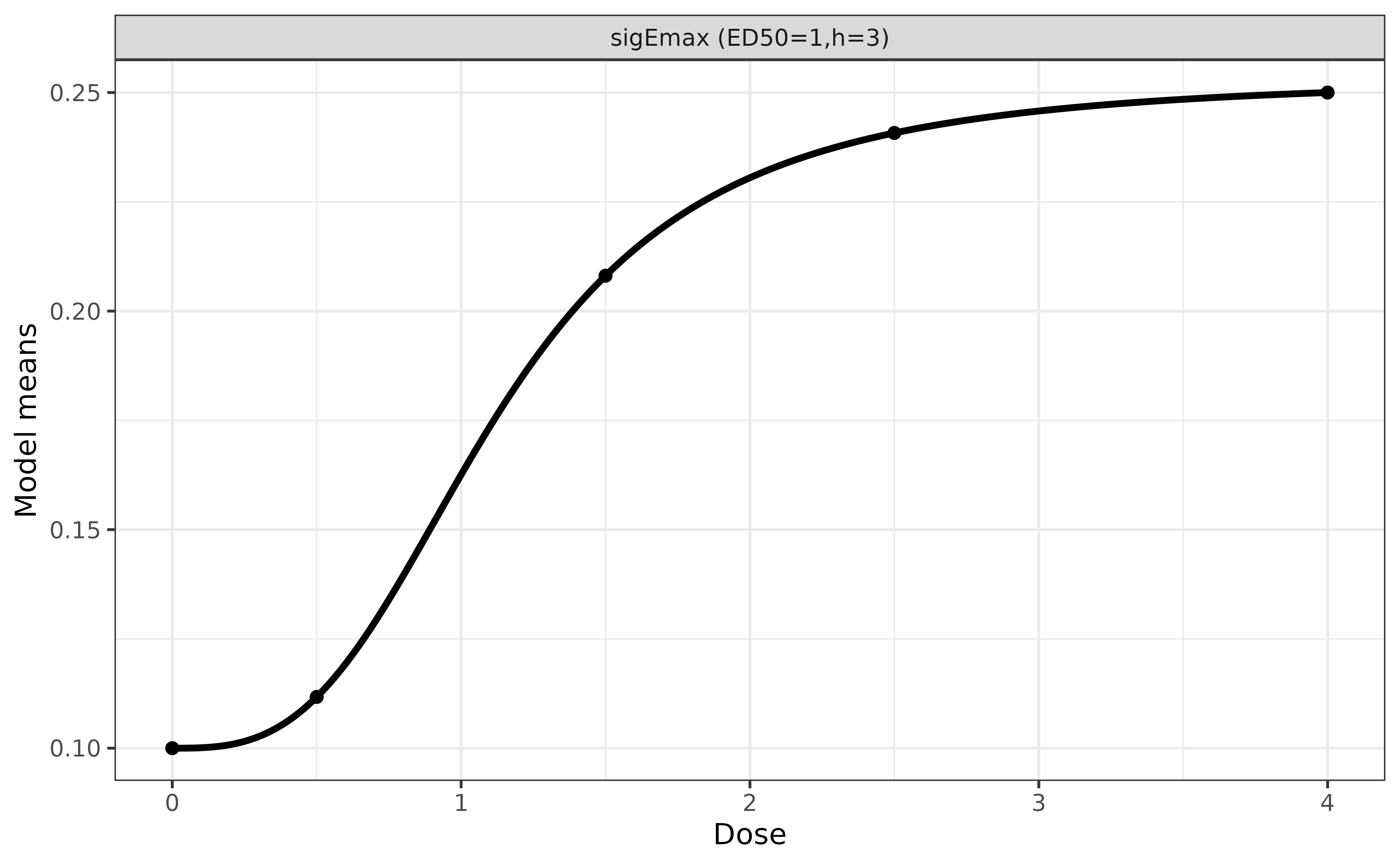
## response rates on curve
x <- DoseFinding::getResp(mods, doses = c(0, 0.5, 1.5, 2.5, 4))
1 / (1 + exp(-unclass(x)))
#>      sigEmax1
#> 0   0.1000000
#> 0.5 0.1117242
#> 1.5 0.2080893
#> 2.5 0.2407520
#> 4   0.2500000
#> attr(,"parList")
#> attr(,"parList")$sigEmax1
#>        e0      eMax      ed50         h
#> -2.197225  1.115778  1.000000  3.000000
Simulation Settings
In our simulation, we assume
- the response rates of binary endpoint as
| Dose | 0 | 0.5 | 1.5 | 2.5 | 4 |
|---|---|---|---|---|---|
| Response Rate (%) | 10.0 | 11.2 | 20.8 | 24.1 | 25.0 |
- readout time is 1 week.
- no dropout.
- starting with a placebo arm and a treatment arm of the highest dose
(= 4), with a 1:1 randomization ratio.
- enroll 5 patients per week for 7 weeks.
- an interim is planed when we have collected 30 readouts in total
from the two arms.
- if z statistic of odds ratio is greater than 1
- add three arms of dose 0.5, 1.5, and 2.5 to trial
- enroll 20 patients per week with a randomization ratio 1:2:2:2:1, until in total 150 patients are enrolled in the trial
- final analysis is performed when readouts are available for all enrolled patients.
- otherwise, stop the trial.
- if z statistic of odds ratio is greater than 1
Define Placebo and High Dose Arms
ep <- endpoint(name = 'ep', type = 'non-tte', readout = c(ep = 1),
               generator = rbinom, size = 1, prob = 0.1)
pbo <- arm(name = 'dose = 0.0')
pbo$add_endpoints(ep)

ep <- endpoint(name = 'ep', type = 'non-tte', readout = c(ep = 1),
               generator = rbinom, size = 1, prob = 0.25)
trt4 <- arm(name = 'dose = 4.0')
trt4$add_endpoints(ep)
Define a Trial
accrual_rate <- data.frame(end_time = c(7, Inf),
                           piecewise_rate = c(5, 20))

trial <- trial(name = '123', n_patients = 150, duration = 14,
               enroller = StaggeredRecruiter, accrual_rate = accrual_rate,
               silent = TRUE)

trial$add_arms(sample_ratio = c(1, 1), pbo, trt4)
trial
#>  ⚕⚕         Trial Name:  123
#>  ⚕⚕        Description:  123
#>  ⚕⚕     Number of Arms:  2
#>  ⚕⚕    Registered Arms:  dose = 0.0, dose = 4.0
#>  ⚕⚕       Sample Ratio:  1, 1
#>  ⚕⚕ Number of Patients:  150
#>  ⚕⚕   Planned Duration:  14
#>  ⚕⚕            Regimen:  not set
#>  ⚕⚕        Random Seed:  1960520344
Define Milestones and Actions
Two milestones are triggered when 30 and 150 readouts are collected, respectively. Note that the 30 readouts are from the placebo and the highest dose arm, while the 150 readouts are from all five arms.
interim <- milestone(name = 'interim',
                     when = eventNumber(endpoint = 'ep', n = 30),
                     action = action_at_interim)

final <- milestone(name = 'final',
                   when = eventNumber(endpoint = 'ep', n = 150),
                   action = action_at_final)
In the action function action_at_interim(), we don’t
actually terminate the trial in simulation but always add dose arms.
Instead, we save the z statistic for summary later, e.g., computing the
proportion of early termination.
action_at_interim <- function(trial){

  ## get data snapshot
  locked_data <- trial$get_locked_data('interim')

  ## compare two arms
  ## Risk difference = response rate in high dose - response rate in placebo
  fit <- fitLogistic(ep ~ arm, placebo = 'dose = 0.0',
                     data = locked_data, alternative = 'greater',
                     scale = 'risk difference')

  ## for summary of early termination
  trial$save(value = fit$z, name = 'z_value')
  trial$save(value = ifelse(fit$z > 1.64, 'add dose arms', 'stop trial'),
             name = 'interim_decision')

  ## create three dose arms
  ep <- endpoint(name = 'ep', type = 'non-tte', readout = c(ep = 1),
                 generator = rbinom, size = 1, prob = .112)
  trt1 <- arm(name = 'dose = 0.5')
  trt1$add_endpoints(ep)

  ep <- endpoint(name = 'ep', type = 'non-tte', readout = c(ep = 1),
                 generator = rbinom, size = 1, prob = .208)
  trt2 <- arm(name = 'dose = 1.5')
  trt2$add_endpoints(ep)

  ep <- endpoint(name = 'ep', type = 'non-tte', readout = c(ep = 1),
                 generator = rbinom, size = 1, prob = .241)
  trt3 <- arm(name = 'dose = 2.5')
  trt3$add_endpoints(ep)

  ## add three new arms to trial
  trial$add_arms(sample_ratio = c(2, 2, 2), trt1, trt2, trt3)

}
At final analysis, we analyze data from all five arms using MCPMod.
It calls a helper function go_nogo() which can be found in
the Appendix below.
action_at_final <- function(trial){

  locked_data <- trial$get_locked_data('final')

  trial$save(value = go_nogo(locked_data), name = 'decision')

}
Execute a Trial
After registering the two milestones with a listener, we simulate a
single trial using controller$run(). We can see that more
patients are randomized to the three newly added arms after interim,
reflecting the new randomization ratio 1:2:2:2:1.
listener <- listener()
listener$add_milestones(interim, final)

controller <- controller(trial, listener)
controller$run(n = 1, plot_event = TRUE)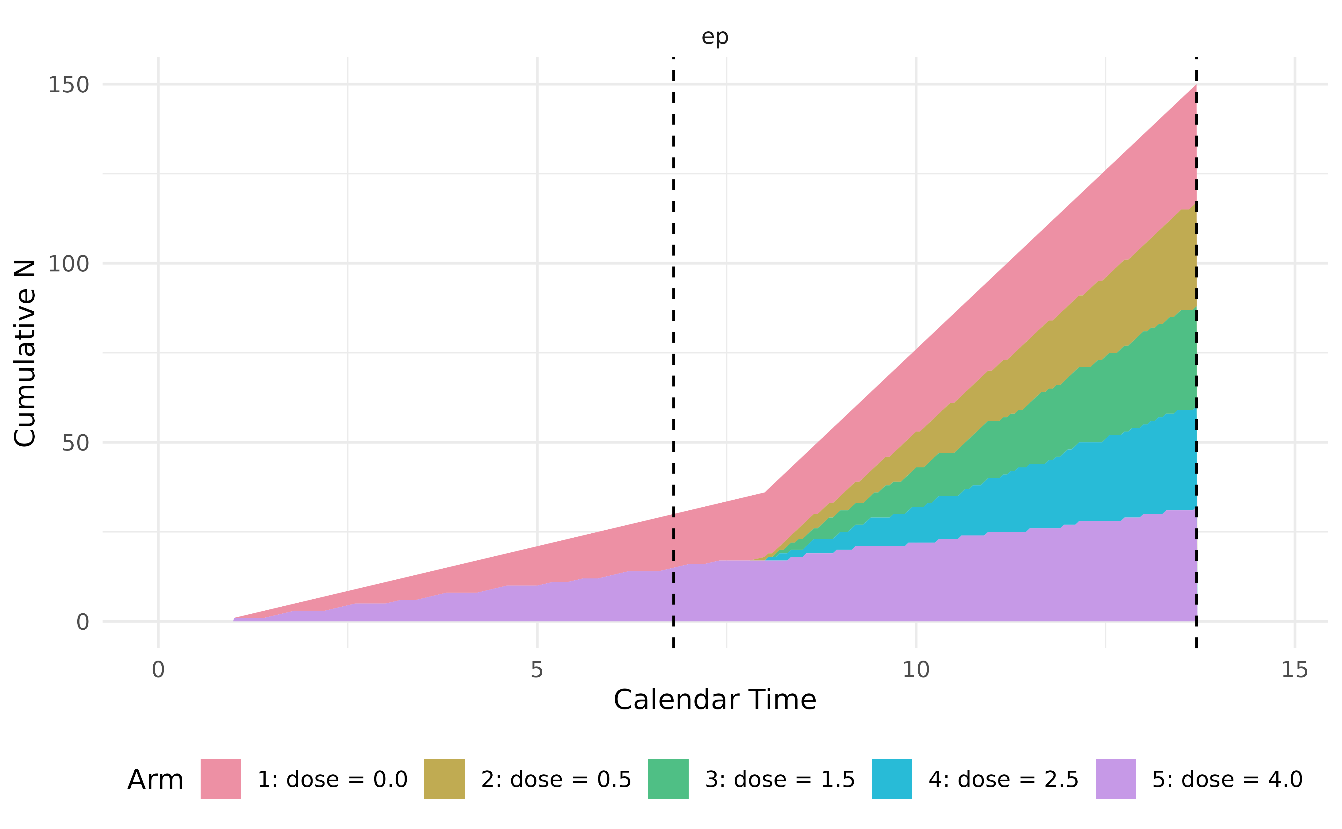
In this trial, the z statistic at interim is relatively low (0.93), thus is early terminated even if in simulation we keep going with three newly added dose arms.
output <- controller$get_output()

output %>%
  kable(escape = FALSE) %>%
  kable_styling(bootstrap_options = "striped",
                full_width = FALSE,
                position = "left") %>%
scroll_box(width = "100%")| trial | seed | milestone_time_<interim> | n_events_<interim>_<ep> | n_events_<interim>_<patient_id> | n_events_<interim>_<arms> | z_value | interim_decision | milestone_time_<final> | n_events_<final>_<ep> | n_events_<final>_<patient_id> | n_events_<final>_<arms> | decision | error_message |
|---|---|---|---|---|---|---|---|---|---|---|---|---|---|
| 123 | 1960520344 | 6.8 | 30 | 35 | c(“dose …. | 0.9258209 | stop trial | 13.7 | 150 | 150 | c(“dose …. | no-go |
We can call controller$run(n = 10) to simulate
additional trials. in the function action_at_final(), the
go/no-go decision (decision in output) is determined under
the assumption that the dose has been expanded, regardless of the
interim evidence—this simplification is made solely for the convenience
of simulation. However, the overall probability of a "go"
should incorporate the interim results—specifically, the trial must not
be stopped at interim (i.e.,
interim_decision == "add dose arms"), and the function
go_nogo() must return "go" at the final
analysis.
## important: reset before calling run() again
controller$reset()
controller$run(n = 10, plot_event = FALSE, silent = TRUE)
res <- controller$get_output()
res %>%
  kable(escape = FALSE) %>%
  kable_styling(bootstrap_options = "striped",
                full_width = FALSE,
                position = "left") %>%
scroll_box(width = "100%")| trial | seed | milestone_time_<interim> | n_events_<interim>_<ep> | n_events_<interim>_<patient_id> | n_events_<interim>_<arms> | z_value | interim_decision | milestone_time_<final> | n_events_<final>_<ep> | n_events_<final>_<patient_id> | n_events_<final>_<arms> | decision | error_message |
|---|---|---|---|---|---|---|---|---|---|---|---|---|---|
| 123 | 1915467752 | 6.8 | 30 | 35 | c(“dose …. | 0.6123731 | stop trial | 13.7 | 150 | 150 | c(“dose …. | go | |
| 123 | 1678009487 | 6.8 | 30 | 35 | c(“dose …. | 0.9258209 | stop trial | 13.7 | 150 | 150 | c(“dose …. | no-go | |
| 123 | 1177293210 | 6.8 | 30 | 35 | c(“dose …. | 0.4918697 | stop trial | 13.7 | 150 | 150 | c(“dose …. | no-go | |
| 123 | 155620919 | 6.8 | 30 | 35 | c(“dose …. | 1.3327856 | stop trial | 13.7 | 150 | 150 | c(“dose …. | go | |
| 123 | 1745672662 | 6.8 | 30 | 35 | c(“dose …. | 1.2247450 | stop trial | 13.7 | 150 | 150 | c(“dose …. | go | |
| 123 | 484372378 | 6.8 | 30 | 35 | c(“dose …. | 1.9364930 | add dose arms | 13.7 | 150 | 150 | c(“dose …. | go | |
| 123 | 2788507 | 6.8 | 30 | 35 | c(“dose …. | 0.4330129 | stop trial | 13.7 | 150 | 150 | c(“dose …. | no-go | |
| 123 | 1945408685 | 6.8 | 30 | 35 | c(“dose …. | 0.4918697 | stop trial | 13.7 | 150 | 150 | c(“dose …. | no-go | |
| 123 | 737764402 | 6.8 | 30 | 35 | c(“dose …. | 0.9258209 | stop trial | 13.7 | 150 | 150 | c(“dose …. | go | |
| 123 | 787086561 | 6.8 | 30 | 35 | c(“dose …. | 1.0954461 | stop trial | 13.7 | 150 | 150 | c(“dose …. | go |
Appendix: Code of Helper Function
For completeness, the full code of the helper functions
go_nogo() is included below, which informs go/no-go
decision at the end of the trial.
go_nogo <- function(data){

  ## candidate models for MCPMod
  doses <- c(0, 0.5, 1.5, 2.5, 4)
  candidates <- Mods(emax = c(.25, 1),
                     sigEmax = rbind(c(1, 3), c(2.5, 4)),
                     betaMod = c(1.1, 1.1),
                     placEff = log(.1/(1 - .1)),
                     maxEff = log(.25/(1 - .25)) - log(.1/(1 - .1)),
                     doses = doses)

  fit <- glm(ep ~ factor(arm) + 0, data = data, family = binomial)
  mu_hat <- coef(fit)
  S_hat <- vcov(fit)

  ## multiple contrast test
  test <- DoseFinding::MCTtest(dose = doses,
                               mu_hat, S = S_hat,
                               models = candidates, type = "general")

  ## model averaging
  model <- DoseFinding::maFitMod(dose = doses,
                                 mu_hat, S = S_hat,
                                 models = c("emax", "sigEmax", "betaMod"))

  ## predict response rate per dose
  prd <- predict(model, summaryFct = median, doseSeq = doses)

  ## convert to scale of probability
  prd_rate <- 1 / (1 + exp(-prd))

  ## go/no-go rule: MCP test p-value < 0.05 and estimated effect > 10%
  ifelse(min(attr(test$tStat, 'pVal')) < .05 &
           max(prd_rate - prd_rate[1]) > .1, 'go', 'no-go')

}