Simulate Correlated Progression-Free Survival and Overall Survival as Endpoints in Clinical Trials

Progression-free survival (PFS) and overall survival (OS) are commonly used as confirmatory endpoints in clinical trials. These two endpoints are typically highly correlated, and it is always the case that PFS $\leq$ OS. A reliable algorithm for simulating both PFS and OS is therefore of great interest.

Several methods have been proposed to achieve this, but many rely on latent variables or copula-based approaches, making it difficult to interpret and specify model parameters in practical settings. In this vignette, we do not aim to provide a comprehensive review of existing methods. Instead, we focus on a three-state illness-death model consisting of the following states: initial (0), progression (1), and death (2). For more details, refer to Meller, Beyersmann, and Rufibach (2019).

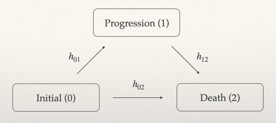
We consider the simplest case of the illness-death model, where all transition hazards $h(t)$ are constant over time. A data generator of this model is implemented in TrialSimulator::CorrelatedPfsAndOs3(), which can be used to define endpoints in TrialSimulator::endpoint().

Marginally, the survival functions of PFS and OS are given by

$$\Pr(\mbox{PFS} > t) = \exp\{-(h_{01} + h_{02})t\}$$

and

$$\Pr(\mbox{OS} > t) = \exp\{-(h_{01} + h_{02})t\} + \frac{h_{01}}{h_{12}-h_{01}-h_{02}}\exp\{-(h_{01} + h_{02})t\} - \exp\{-h_{12}t\}$$

Thus, PFS follows an exponential distribution with rate $h_{01} + h_{02}$, which is also referred to as the all-cause hazard. Given the transition hazards $h_{01}, h_{02}, h_{12}$, a patient’s trajectory can be simulated using the following algorithm:

• Step 1. Generate the time to progression $t_{01}$ from an exponential distribution with rate $h_{01} + h_{02}$.

• Step 2. Draw a Bernoulli sample with success probability $\frac{h_{02}}{h_{01} + h_{02}}$. If successful, the patient dies immediately, i.e., time to death $t_{02} = t_{01}$, and the simulation ends. Otherwise, proceed to Step 3.

• Step 3. Generate the time from progression to death $t_{12}$ from an exponential distribution with rate $h_{12}$. Then, time to death $t_{02} = t_{01} + t_{12}$, and the simulation ends.

Reparameterization

Although statistical methods exist for estimating transition hazards when data are available (e.g., the R package simIDM), in simulation studies for trial planning, it is common to specify these hazard parameters based on limited information. A more intuitive way to define PFS and OS is through their medians and correlation coefficient. In this section, we describe a reparameterization strategy that maps the medians and correlation to the transition hazards.

Let $m_1$ and $m_2$ denote the medians of PFS and OS, respectively. Then we have

$$h_{01} + h_{02} = \frac{\log(2)}{m_1} \tag{1}$$

and

$$\frac{1}{2} = \exp\{-(h_{01} + h_{02})m_2\} + \frac{h_{01}}{h_{12}-h_{01}-h_{02}}\exp\{-(h_{01} + h_{02})m_2\} - \exp\{-h_{12}m_2\}$$ Through algebraic manipulation, we obtain

$$h_{01} = \frac{(\frac{1}{2} - \exp\{-\log(2) \frac{m_2}{m_1}\}) (h_{12} - \log(2) \frac{1}{m_1})}{ (\exp\{-\log(2) \frac{m_2}{m_1}\} - \exp\{-h_{12} m_2\})} \tag{2}$$

This implies that, for given medians $m_1$ and $m_2$, we can perform a grid search over values of $h_{12}$. For each candidate value, we compute $h_{01}$ and $h_{02}$ using equations (1) and (2), respectively. Then, we simulate a large dataset using TrialSimulator::CorrelatedPfsAndOs3() and calculate the Pearson correlation between PFS and OS. We select the value of $h_{12}$ (and the corresponding $h_{01}, h_{02}$) that yields the desired correlation.

This reparameterization of the three-state illness-death model enables us to specify correlated PFS and OS based on their medians and correlation, which is more interpretable and practical in clinical trial design. The TrialSimulator package provides a dedicated function, solveThreeStateModel, to facilitate this process.

Example

Suppose we aim to simulate PFS with a median of 5 and OS with a median of 12, targeting a correlation of 0.6 between them.

pars <- solveThreeStateModel(median_pfs = 5, median_os = 12, 
                             corr = seq(.55, .65, by = .05), 
                             h12 = seq(.05, .15, length.out = 50))
plot(pars)
#>   corr       h01        h02        h12       error
#> 1 0.55 0.0997785 0.03885093 0.08877551 0.001158721
#> 2 0.60 0.1080742 0.03055522 0.10102041 0.003826014
#> 3 0.65 0.1214222 0.01720720 0.11938776 0.004866790
#> Warning: Removed 3 rows containing missing values or values outside the scale range
#> (`geom_segment()`).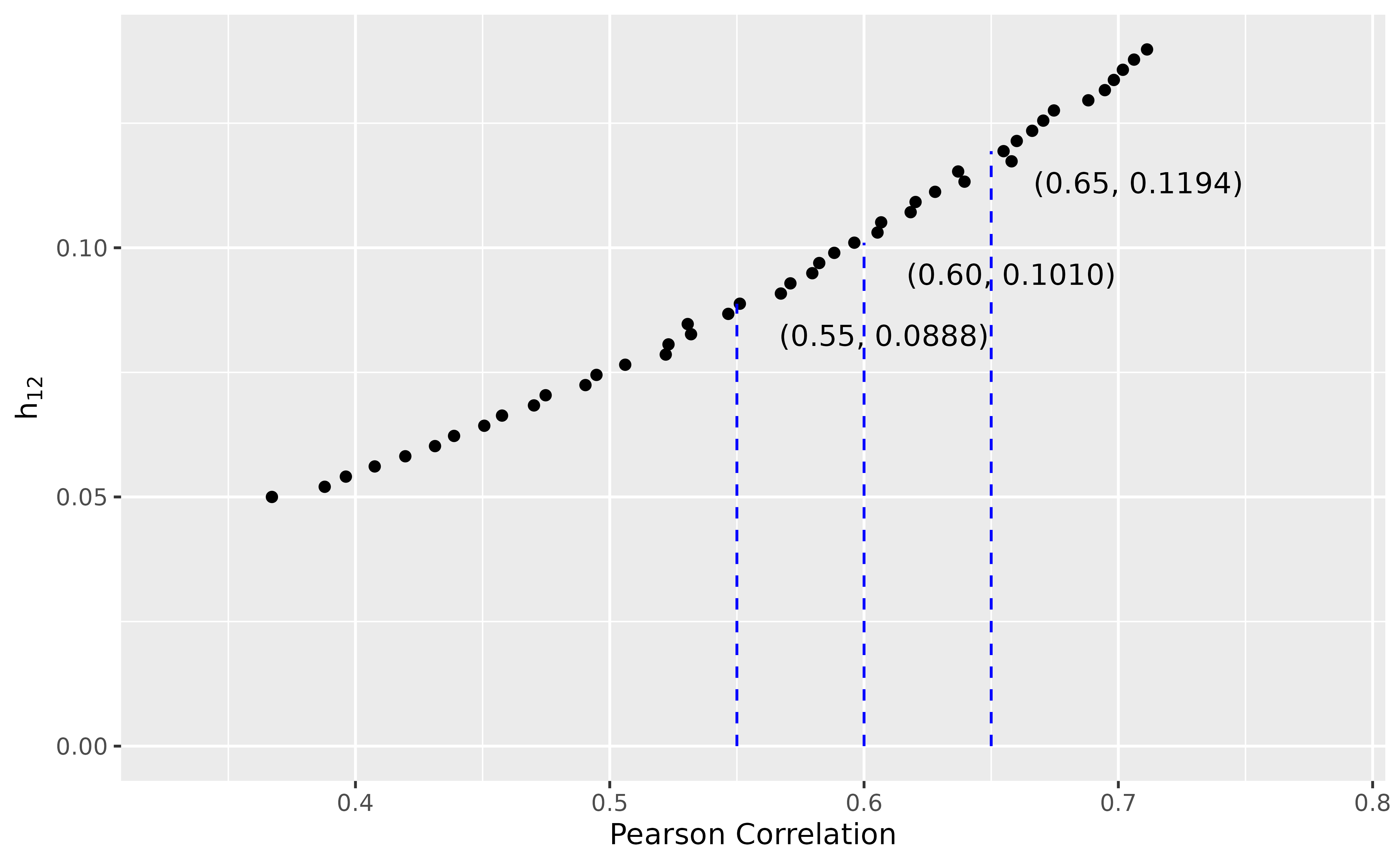

The result suggests that using $h_{01} = 0.11$, $h_{02} = 0.03$, and $h_{12} = 0.10$ may achieve the desired specifications. To verify this, we simulate PFS and OS data using

pfs_and_os <- endpoint(name = c('pfs', 'os'), 
                       type = c('tte', 'tte'), 
                       generator = CorrelatedPfsAndOs3, 
                       h01 = .11, h02 = .03, h12 = .10, 
                       pfs_name = 'pfs', os_name = 'os')
pfs_and_os

If you are not familiar with the TrialSimulator framework, you can generate PFS and OS directly by calling CorrelatedPfsAndOs3():

dat <- CorrelatedPfsAndOs3(n = 1e6, h01 = .11, h02 = .03, h12 = .10)
head(dat, 2)
#>        pfs        os pfs_event os_event
#> 1 4.263915 12.997581         1        1
#> 2 4.257848  4.257848         1        1

## should be close to 0.6
with(dat, cor(pfs, os))
#> [1] 0.58961

## should be close to 5.0
with(dat, median(pfs))
#> [1] 4.965547

## should be close to 12.0
with(dat, median(os))
#> [1] 12.06319
with(dat, all(pfs <= os))
#> [1] TRUE

Further Discussion

In this vignette, we demonstrate how to derive the transition hazards from the medians of PFS and OS, along with their Pearson correlation coefficient. It is important to note that the correlation is computed based on data simulated from the specified hazard, and therefore can be substituted by any other measure that is relevant to the simulation objective.

For instance, one may simulate trial data for two treatment arms, each defined by their own PFS and OS medians and $h_{12}$. Instead of using the correlation between simulated PFS and OS times, one could compute the correlation between the $z$-statistics from the respective treatment comparisons of PFS and OS. This alternative approach may be more appropriate in scenarios where the joint behavior of test statistics, rather than raw survival times, is of primary interest—such as in the context of multiple testing or endpoint selection.