Designs with Response-Adaptive Randomization

Response-adaptive randomization (RAR) can be a powerful strategy in Phase II dose-finding trials. It allows sponsors to dynamically update the randomization scheme at one or more interim analyses based on accumulating data. By shifting allocation toward more promising treatment arms, RAR can enhance the ethical and statistical efficiency of the trial.

This vignette demonstrates how to simulate a trial with response-adaptive design using the TrialSimulator package. For further background, refer to this document from the MedianaDesigner package. Dr. Alex Dmitrienko also provides a series of excellent online lectures on this topic:

Part 1
Part 2.

However, the original MedianaDesigner::ADRand() function is no longer functional, even for examples provided on this page. Therefore, this vignette focuses on implementing a similar response-adaptive design using TrialSimulator. The core algorithm for updating the randomization ratio is re-implemented based on the logic of the DoseFinding package and may differ slightly from that used in Dr. Dmitrienko’s materials.

Simulation Settings

We assume an Emax model for the endpoint fev1 (forced expiratory volume in 1 second) measured after 4 months of treatment. The maximum effect (0.1) is achieved at dose 100.
The trial includes one placebo arm and five active arms with doses: 20, 25, 30, and 35.
- Patients are initially randomized equally across all five arms.
A total of 200 patients are recruited over 36 months, with 50% of enrollment expected by 24 months.
Two interim analyses are planned after 50 and 120 patients have non-missing fev1 readouts, i.e. pipeline patients are excluded.
The final analysis is performed when data from all 200 patients are available.
At each interim:
- Candidate dose-response models Emax, sigEmax, and quadratic are fitted.
- Bootstrap estimates from DoseFinding::maFitMod() are used to calculate, for each dose $d \in \{20, 25, 30, 35\}$ , the probability $p_d$ that the estimated treatment effect exceeds 0.08.
- The randomization ratio for each active dose is set proportional to $p_d$
- The placebo ratio remains fixed at 20%.
At the final analysis, a multiple contrast test is conducted using data from all 200 patients.

Define Data Generator of `fev1`

The following function generates fev1 outcomes using the assumed Emax model. It is later assigned as the generator function when defining endpoints.

rng <- function(n, dose){

  model <- DoseFinding::Mods(
    emax = c(2.6, 12.5),
    placEff = 1.25, maxEff = 0.1,
    doses = c(0, 20, 25, 50, 100))

  data.frame(
    fev1 = rnorm(n, mean = getResp(model, doses = dose), sd = .05)
  )

}

Define `fev1` Endpoints for Each Arm

Each treatment arm is associated with an endpoint definition, specifying the dose and data generator.

fev1 <- endpoint(name = 'fev1', type = 'non-tte', readout = c(fev1 = 4),
                 generator = rng, dose = 0)
pbo <- arm(name = '0.0')
pbo$add_endpoints(fev1)

fev1 <- endpoint(name = 'fev1', type = 'non-tte', readout = c(fev1 = 4),
                 generator = rng, dose = 20.0)
dose1 <- arm(name = '20.0')
dose1$add_endpoints(fev1)

fev1 <- endpoint(name = 'fev1', type = 'non-tte', readout = c(fev1 = 4),
                 generator = rng, dose = 25.0)
dose2 <- arm(name = '25.0')
dose2$add_endpoints(fev1)

fev1 <- endpoint(name = 'fev1', type = 'non-tte', readout = c(fev1 = 4),
                 generator = rng, dose = 30.0)
dose3 <- arm(name = '30.0')
dose3$add_endpoints(fev1)

fev1 <- endpoint(name = 'fev1', type = 'non-tte', readout = c(fev1 = 4),
                 generator = rng, dose = 35.0)
dose4 <- arm(name = '35.0')
dose4$add_endpoints(fev1)

Define a Trial

Here we define the trial object with 200 patients and an accrual period of 36 months. The total trial duration is extended to 40 months to account for a 4-month follow-up after last enrollment.

accrual_rate <- data.frame(end_time = c(24, Inf),
                           piecewise_rate = c(100/24, 100/12))
trial <- trial(
  name = 'Trial-3415', n_patients = 200,
  seed = 1727811904, duration = 40,
  enroller = StaggeredRecruiter, accrual_rate = accrual_rate
)

trial$add_arms(sample_ratio = rep(1, 5), pbo, dose1, dose2, dose3, dose4)
#> Arm(s) <0.0, 20.0, 25.0, 30.0, 35.0> are added to the trial.
#> Randomization is done for 200 potential patients.
#> Data of 200 potential patients are generated for the trial with 5 arm(s) <0.0, 20.0, 25.0, 30.0, 35.0>.
trial
#>  ⚕⚕ Trial Name:  Trial-3415  
#>  ⚕⚕ Description:  Trial-3415  
#>  ⚕⚕ # of Arms:  5  
#>  ⚕⚕ Registered Arms:  0.0, 20.0, 25.0, 30.0, 35.0  
#>  ⚕⚕ Sample Ratio:  1, 1, 1, 1, 1  
#>  ⚕⚕ # of Patients:  200  
#>  ⚕⚕ Planned Duration:  40  
#>  ⚕⚕ Random Seed:  1727811904

Define Milestones and Associated Actions

Three milestones are defined: two interim analyses and one final analysis. The same action is used for both interims, while a separate one is used for the final.

stage1 <- milestone(name = 'stage 1',
                    when = eventNumber('fev1', n = 50),
                    action = stage_action)

stage2 <- milestone(name = 'stage 2',
                    when = eventNumber('fev1', n = 120),
                    action = stage_action)

final <- milestone(name = 'final',
                   when = eventNumber('fev1', n = 200),
                   action = final_action)

The stage_action() function is called at each interim milestone to lock current data and update sample ratios based on model-based probabilities. It utilities a helper function compute_sample_ratio() which can be found in the Appendix below.

stage_action <- function(trial, milestone_name){

  locked_data <- trial$get_locked_data(milestone_name)
  new_sample_ratio <- compute_sample_ratio(locked_data)

  trial$update_sample_ratio(arm_names = c('0.0', '20.0', '25.0', '30.0', '35.0'),
                            sample_ratios = new_sample_ratio)
  
  message(milestone_name, ': ')
  data.frame(table(locked_data$arm), new_sample_ratio) %>%
    setNames(c('dose', 'total_n', 'new_ratio')) %>% print()

  invisible(NULL)

}

At the final milestone, the function final_action() performs the multiple contrast test and stores the result. It calls a helper function multiple_contrast_test(), which can be found in the Appendix below.

final_action <- function(trial, milestone_name){

  locked_data <- trial$get_locked_data(milestone_name)
  
  message('final: ')
  data.frame(table(locked_data$arm)) %>%
    setNames(c('dose', 'total_n')) %>% print()

  trial$save(value = multiple_contrast_test(locked_data),
             name = 'MC_test')

  invisible(NULL)
}

Execute a Trial

After registering all milestones with a listener object, we simulate the trial using controller$run().

listener <- listener()
listener$add_milestones(stage1, stage2, final)
#> A milestone <stage 1> is registered.
#> A milestone <stage 2> is registered.
#> A milestone <final> is registered.

controller <- controller(trial, listener)
controller$run(n = 1, plot_event = TRUE, silent = TRUE)
#> stage 1:
#>   dose total_n new_ratio
#> 1  0.0      13 0.2000000
#> 2 20.0      13 0.1056760
#> 3 25.0      13 0.1469556
#> 4 30.0      14 0.2253870
#> 5 35.0      13 0.3219814
#> stage 2:
#>   dose total_n  new_ratio
#> 1  0.0      31 0.20000000
#> 2 20.0      25 0.03908046
#> 3 25.0      26 0.10344828
#> 4 30.0      28 0.21839080
#> 5 35.0      43 0.43908046
#> final:
#>   dose total_n
#> 1  0.0      40
#> 2 20.0      26
#> 3 25.0      32
#> 4 30.0      39
#> 5 35.0      63

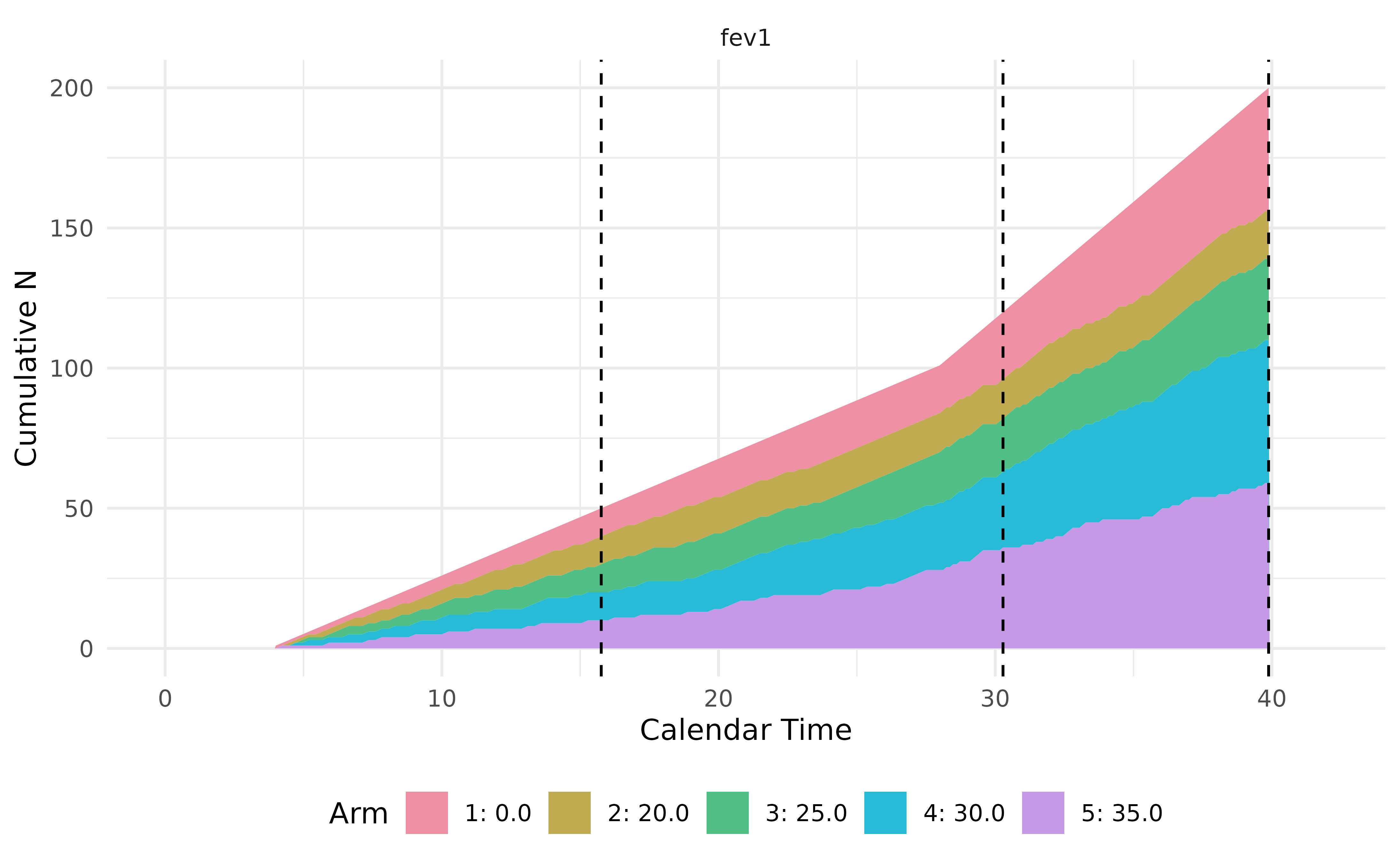
output <- controller$get_output()

output %>% 
  kable(escape = FALSE) %>% 
  kable_styling(bootstrap_options = "striped", 
                full_width = FALSE,
                position = "left") %>%
  scroll_box(width = "100%")

trial	seed	milestone_time_<stage 1>	n_events_<stage 1>_<patient_id>	n_events_<stage 1>_<fev1>	n_events_<stage 1>_<arms>	milestone_time_<stage 2>	n_events_<stage 2>_<patient_id>	n_events_<stage 2>_<fev1>	n_events_<stage 2>_<arms>	milestone_time_<final>	n_events_<final>_<patient_id>	n_events_<final>_<fev1>	n_events_<final>_<arms>	MC_test	error_message
Trial-3415	1727811904	15.76	66	50	c(13, 10….	30.28	153	120	c(31, 24….	39.88	200	200	c(40, 40….	TRUE

In the output, the columns n_event_<milestone>_<arms> contain detailed information on observed events or sample sizes per arm at each milestone. It is evident that we have pipeline patients at both interims.

output[, 'n_events_<stage 1>_<arms>']
#> [[1]]
#>   X0.0 X20.0 X25.0 X30.0 X35.0   endpoint
#> 1   13    13    13    14    13 patient_id
#> 2   10    10    10    10    10       fev1

output[, 'n_events_<stage 2>_<arms>']
#> [[1]]
#>   X0.0 X20.0 X25.0 X30.0 X35.0   endpoint
#> 1   31    25    26    28    43 patient_id
#> 2   24    20    23    23    30       fev1

output[, 'n_events_<final>_<arms>']
#> [[1]]
#>   X0.0 X20.0 X25.0 X30.0 X35.0   endpoint
#> 1   40    26    32    39    63 patient_id
#> 2   40    26    32    39    63       fev1

Appendix: Codes of Helper Functions

For completeness, the full code of the helper functions compute_sample_ratio() and multiple_contrast_test() is included below, which determine the new sample ratio and performs the multiple contrast test.

compute_sample_ratio <- function(data){

  data$dose <- as.numeric(data$arm)
  fit <- lm(fev1 ~ factor(dose) - 1, data = data)
  dose <- unique(sort(data$dose))
  mu_hat <- coef(fit)
  S_hat <- vcov(fit)

  suppressMessages(
    ma_fit <- DoseFinding::maFitMod(dose, mu_hat, S = S_hat,
                                    models = c("emax", "sigEmax", "quadratic"))
  )

  pred <- predict(ma_fit, doseSeq = c(0, 20, 25, 30, 35), summaryFct = NULL)
  prob <- apply(pred[, -1] - pred[, 1], 2, function(x){mean(x > .08)})
  sample_ratio <- c(.2, (1 - .2) * prob / sum(prob)) %>% unname()

  sample_ratio
}

multiple_contrast_test <- function(data){
  
  candidate_models <- DoseFinding::Mods(
    emax = c(2.6, 12.5), sigEmax = c(30.5, 3.5), quadratic = -0.00776,
    placEff = 1.25, maxEff = 0.15, doses = c(0, 20, 25, 30, 35))

  data$dose <- as.numeric(data$arm)
  test <- DoseFinding::MCTtest(dose = dose, resp = fev1,
                               models = candidate_models, data = data)
  
  ## at least one dose shows significant non-flatten pattern
  any(attr(test$tStat, 'pVal') < .05)

}