Define Non-Time-to-Event Endpoints in Clinical Trials • TrialSimulator

TrialSimulator provides a flexible framework for defining and simulating a variety of clinical trial endpoints by specifying the type parameter in endpoints. This vignette covers non-time-to-event (non-TTE) endpoints, demonstrating how they can be defined, integrated into trial arms, and analyzed at pre-specified milestone triggers. For time-to-event endpoints, please refer to the vignette Define Time-to-Event Endpoints in Clinical Trials.

This vignette demonstrates how to use the following key functions to define time-to-event endpoints. For the sake of completeness, we also demonstrates how to define arms and trial with the created endpoints

endpoint: Creates one or more endpoints
test_generator: Generates an example dataset from an Endpoint object
arm: Creates one or more arms
add_endpoints: Add one or more endpoints into an arm
milestone: Defines one or more milestones when data snapshots are created for analysis

Define endpoints with random number generators

Similar to time-to-event endpoints, non-TTE endpoints can be defined using any univariate random number generator that takes n (number of observations) as its first argument. The stats package provides a set of random number generators that can be assigned to generator in endpoints, where additional arguments required by generator can be passed through .... When creating non-TTE endpoints, the argument type should be set to "non-tte", and the argument readout should be specified as a named numeric vector, indicating the time required for the endpoint to be available for analysis after patient enrollment.

In the example below, we define two types of endpoints:

Continuous endpoint: Tumor size change from baseline (cfb), available after 6 months, assuming a normal distribution (generator = rnorm) with custom mean and sd.
Binary endpoint: Objective response rate (orr), available after 2 months, assuming a binomial distribution (generator = rbinom) with size = 1 and custom prob.

## endpoints in placebo arm
tumor_cfb_pbo <- endpoint(name = 'cfb', type = 'non-tte', 
                          readout = c(cfb = 6),
                          generator = rnorm, mean = .8, sd = 3.2)
orr_pbo <- endpoint(name = 'orr', type = 'non-tte', 
                    readout = c(orr = 2),
                    generator = rbinom, size = 1, prob = .1)

## define the placebo arm
pbo <- arm(name = 'placebo')
pbo$add_endpoints(tumor_cfb_pbo, orr_pbo)

## endpoints in treatment arm
tumor_cfb_trt <- endpoint(name = 'cfb', type = 'non-tte', 
                          readout = c(cfb = 6), 
                          generator = rnorm, mean = -2.3, sd = 1.5)
orr_trt <- endpoint(name = 'orr', type = 'non-tte', 
                    readout = c(orr = 2), 
                    generator = rbinom, size = 1, prob = .25)

## define the treatment arm
trt <- arm(name = 'treatment')
trt$add_endpoints(tumor_cfb_trt, orr_trt)

With the treatment arms defined, we can proceed to create a trial. Patients are recruited at a piecewise constant rate, with an accrual pattern as follows:

First 6 months: 10 patients per month.
After 6 months: 20 patients per month until 420 patients are randomized 1:1 into the two arms.

We also specify a dropout process with a Weibull distribution. The dropout rates are set as follows:

15% dropout at 12 months
30% dropout at 18 months

These constraints are resolved using the Weibull dropout function:

$\begin{split} 0.15 & = & 1 - e^{-(12/\lambda)^k} \\ 0.30 & = & 1 - e^{-(18/\lambda)^k} \end{split}$

dropout_pars <- weibullDropout(c(12, 18), c(.15, .30))
dropout_pars
#>     shape     scale 
#>  1.938589 30.635696

Using the computed scale parameter $\lambda=$ 30.636 and shape parameter $k=$ 1.939, we specify the trial setup:

accrual_rate <- data.frame(end_time = c(6, Inf), 
                           piecewise_rate = c(10, 20))

trial <- trial(
  name = 'Trial-31415', description = 'Example Clinical Trial', 
  n_patients = 420, duration = 30, 
  enroller = StaggeredRecruiter, accrual_rate = accrual_rate, 
  dropout = rweibull, scale = 30.636, shape = 1.939
)
#> Seed is not specified. TrialSimulator sets it to 1012203595

## add arms to the trial
trial$add_arms(sample_ratio = c(1, 1), trt, pbo)
#> Arm(s) <treatment, placebo> are added to the trial.
#> Randomization is done for 420 potential patients.
#> Data of 420 potential patients are generated for the trial with 2 arm(s) <treatment, placebo>.
trial
#>  ⚕⚕ Trial Name:  Trial-31415  
#>  ⚕⚕ Description:  Example Clinical Trial  
#>  ⚕⚕ # of Arms:  2  
#>  ⚕⚕ Registered Arms:  treatment, placebo  
#>  ⚕⚕ Sample Ratio:  1, 1  
#>  ⚕⚕ # of Patients:  420  
#>  ⚕⚕ Planned Duration:  30  
#>  ⚕⚕ Random Seed:  1012203595

Here accrual_rate is an argument of TrialSimulator::StaggeredRecruiter controlling how patients are recruited into the trial. Similarly, scale and shape are arguments of rweibull. All these arguments are passed through ... of trial().

TrialSimulator allows defining trial milestones at specific time points when data is locked for analysis. Here, we define three key milestones:

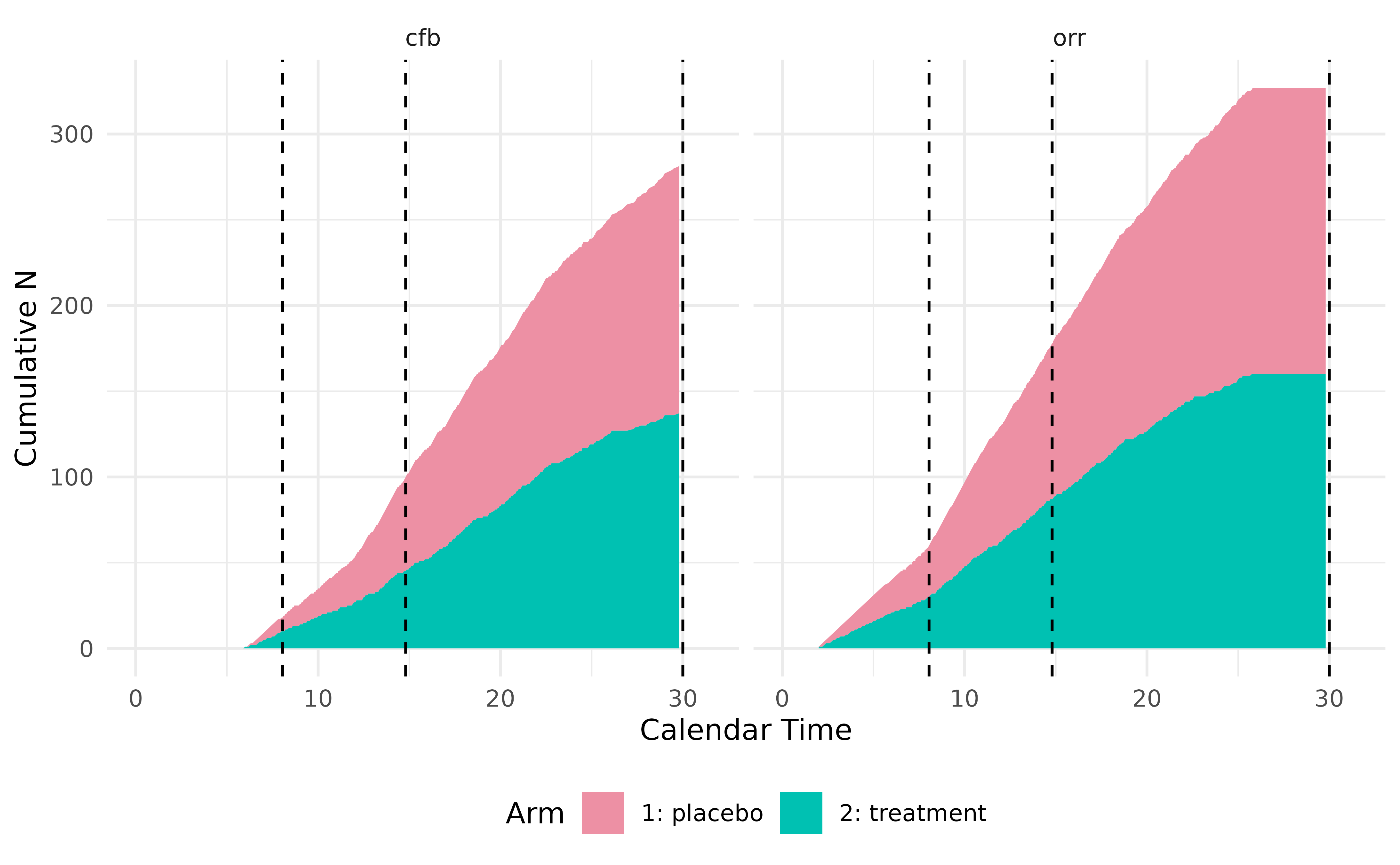
Interim Analysis: Triggered when orr has been observed for 60 patients.
Random Checkpoint: For illustration purpose only. Triggered when the trial has reached at least 10 months, and at least one of the following conditions is met:
- cfb has been observed for at least 100 patients,
- orr has been observed for at least 180 patients.
Final Analysis: Occurs when the trial reaches 30 months.

interim <- milestone(name = 'interim', 
                     trigger_condition = eventNumber(endpoint = 'orr', n = 60), 
                     action = doNothing)

random <- milestone(name = 'random', 
                    trigger_condition = 
                      calendarTime(time = 10) & 
                      (eventNumber(endpoint = 'cfb', n = 100) | 
                         eventNumber(endpoint = 'orr', n = 180)
                       ), 
                    action = doNothing)

final <- milestone(name = 'final', 
                   trigger_condition = calendarTime(time = 30), 
                   action = doNothing)

Here action = doNothing in milestone means we don’t expect any action at the time of triggered milestones. In practice, instead of doNothing, custom action function can be adopted to add or remove arms (e.g., dose selection), adjust sample ratio per arm, or carry out statistical analysis based on locked data. These advanced setups are covered in other vignettes.

Next, we register the milestones with a listener and create a controller to monitor and execute the trial.

## register milestones to the listener
listener <- listener()
listener$add_milestones(interim, random, final)
#> A milestone <interim> is registered.
#> A milestone <random> is registered.
#> A milestone <final> is registered.

## run the trial
controller <- controller(trial, listener)
controller$run()
#> Conditioin of milestone <interim> is being checked.
#> Data is locked at time = 8.05 for milestone <interim>.
#> Locked data can be accessed in Trial$get_locked_data('interim'). 
#> Number of events at lock time:
#>   patient cfb orr                 arms
#> 1     102  18  60 <treatment, placebo>
#> 
#> Conditioin of milestone <random> is being checked.
#> Data is locked at time = 14.8 for milestone <random>.
#> Locked data can be accessed in Trial$get_locked_data('random'). 
#> Number of events at lock time:
#>   patient cfb orr                 arms
#> 1     237 100 178 <treatment, placebo>
#> 
#> Conditioin of milestone <final> is being checked.
#> Data is locked at time = 30 for milestone <final>.
#> Locked data can be accessed in Trial$get_locked_data('final'). 
#> Number of events at lock time:
#>   patient cfb orr                 arms
#> 1     420 282 327 <treatment, placebo>
#>

We can inspect the dataset locked at different milestone by calling member function get_locked_data with milestone names. Ideally, this should be done within custom action function, where decision is made based on data locked at the time of a milestone.

interim_data <- trial$get_locked_data(milestone_name = 'interim')
random_data <- trial$get_locked_data(milestone_name = 'random')
final_data <- trial$get_locked_data(milestone_name = 'final')
head(interim_data)
#>   patient_id       arm enroll_time dropout_time       cfb cfb_readout orr
#> 1          1 treatment         0.0    21.180883 -4.434289           6   0
#> 2          2   placebo         0.1     2.977640        NA           6   0
#> 3          3   placebo         0.2    28.175451 -1.657398           6   1
#> 4          4 treatment         0.3    27.254577  1.004898           6   0
#> 5          5 treatment         0.4     5.663727        NA           6   0
#> 6          6   placebo         0.5    27.379476  6.093597           6   0
#>   orr_readout
#> 1           2
#> 2           2
#> 3           2
#> 4           2
#> 5           2
#> 6           2

Since cfb has a 6-month readout time, at interim analysis, some patients’ cfb values are still unavailable, appearing as NA in interim_data. However, these values become available in random_data collected at a later time point. This demonstrates how TrialSimulator properly and automatically handles endpoint availability at different milestones

not_ready_at_interim <- 
  interim_data %>% 
  dplyr::filter(is.na(cfb) & 
                  is.na(orr) & 
                  enroll_time + 6 < dropout_time) %>% 
  head() %>% 
  print()
#>   patient_id       arm enroll_time dropout_time cfb cfb_readout orr orr_readout
#> 1         63 treatment        6.10     23.76025  NA           6  NA           2
#> 2         64   placebo        6.15     29.50080  NA           6  NA           2
#> 3         66   placebo        6.25     26.44169  NA           6  NA           2
#> 4         67   placebo        6.30     25.48133  NA           6  NA           2
#> 5         69   placebo        6.40     84.56996  NA           6  NA           2
#> 6         70 treatment        6.45     31.77506  NA           6  NA           2

random_data %>% 
  dplyr::filter(patient_id %in% not_ready_at_interim$patient_id) %>% 
  print()
#>   patient_id       arm enroll_time dropout_time        cfb cfb_readout orr
#> 1         63 treatment        6.10     23.76025 -4.8136091           6   0
#> 2         64   placebo        6.15     29.50080  1.5471692           6   0
#> 3         66   placebo        6.25     26.44169 -3.1648153           6   0
#> 4         67   placebo        6.30     25.48133 -3.9319150           6   0
#> 5         69   placebo        6.40     84.56996  1.1369365           6   0
#> 6         70 treatment        6.45     31.77506 -0.7169747           6   0
#>   orr_readout
#> 1           2
#> 2           2
#> 3           2
#> 4           2
#> 5           2
#> 6           2

In this example, we simulate tumor size change from baseline (cfb). However, in many trials, it is more appropriate to simulate tumor size at both baseline and follow-up separately to allow for more complex modeling, such as longitudinal or repeated measures analysis. This will be covered in another vignette.

With this flexible setup, TrialSimulator enables efficient endpoint definition, adaptive trial execution, and data monitoring—allowing users to design and simulate clinical trials tailored to specific research needs.