Conditional Power and Event-Number Reassessment

This vignette explains the statistical model and implementation behind Trials$conditionalPower() and Trials$eventNumberReestimationFromConditionalPower() in detail, including the canonical distribution, alternative-direction mapping, effect assumptions, nonmonotone root search, and integer algorithm. Both methods apply to a time-to-event comparison with one interim analysis and one final analysis. They use the interim logrank statistic and event count stored in a triggered milestone.

The mathematical and diagnostic examples first isolate particular features of the two methods. The later sections then implement the promising-zone policy in a milestone action and use it in a complete TrialSimulator simulation program, following the same action-based pattern used for other adaptive and enrichment designs.

Conditional power is a design calculation, not an automatic adaptation rule. In particular, changing a final event target after an unblinded interim can affect type I error. A promising-zone design must be pre-specified and its complete decision rule must be justified and evaluated, usually by simulation.

Statistical setting

Consider one treatment arm compared with placebo. Let

• $d$ be the number of events observed on the two arms at interim;
• $D>d$ be the total number of events at a future final analysis;
• $z$ be the interim logrank z statistic;
• $r$ be the treatment-to-placebo allocation ratio; and
• $\omega=r/(1+r)^2$ be the Schoenfeld information per event.

The package uses the sign convention of fitLogrank(): $z>0$ corresponds to an estimated treatment-to-placebo hazard ratio greater than one. Therefore, when a hazard ratio below one is beneficial, use alternative = "less".

It is convenient to map both alternatives to a lower-tail problem. Define

$$z_* = \begin{cases} z, & \text{alternative = "less"},\\ -z, & \text{alternative = "greater"}, \end{cases} \qquad \theta_* = \begin{cases} \log(h), & \text{alternative = "less"},\\ -\log(h), & \text{alternative = "greater"}, \end{cases}$$

where $h$ is an assumed treatment-to-placebo hazard ratio. On this common scale, a negative $z_*$ or $\theta_*$ favors treatment. The final rejection region is

$$Z_D^* \leq c_\alpha, \qquad c_\alpha=\Phi^{-1}(\alpha).$$

For alternative = "greater", this is equivalent to comparing the original statistic with the upper boundary $\Phi^{-1}(1-\alpha)$.

What alpha means

The argument alpha is the one-sided nominal level corresponding to the planned final critical boundary. It is not necessarily the total design alpha, the cumulative alpha spent by the final look, or the incremental alpha spent at that look. For example, if an upper-tail group-sequential design has final critical value $c$, pass alpha = 1 - pnorm(c).

Conditional power

The member method has the following signature:

trial$conditionalPower(
  milestone, formula, placebo, alternative, alpha, D, effect, ...
)

Write $t=d/D$ for the interim information fraction. Under the canonical independent-increments model, conditional on the observed interim statistic,

$$Z_D^* \mid Z_d^*=z_* \sim N\left\{ \sqrt{t}\,z_* + \theta_*\sqrt{\omega D}(1-t),\;1-t \right\}.$$

It follows that the lower-tail conditional power is

$$CP(D)=\Phi\left[ \frac{ c_\alpha-\sqrt{d/D}\,z_* -\theta_*\sqrt{\omega D}(1-d/D) }{\sqrt{1-d/D}} \right].$$

The implementation provides three choices for the future effect.

A specified hazard ratio

For a positive numeric effect = h, the method uses $\theta_* = \log(h)$ for "less" and $-\log(h)$ for "greater". This separates the assumed future effect from random variation in the interim estimate. It also requires the allocation ratio recorded at the milestone so that $\omega$ can be computed.

The interim trend

For effect = "trend", the interim estimate is extrapolated:

$$\widehat\theta_* = \frac{z_*}{\sqrt{\omega d}}.$$

Substitution cancels $\omega$ and gives

$$CP_{\text{trend}}(D)=\Phi\left[ \frac{c_\alpha-z_*\sqrt{D/d}}{\sqrt{1-d/D}} \right].$$

This calculation is often useful as a sensitivity analysis, but it can be optimistic after a favorable interim because it treats the noisy interim estimate as the true future effect.

The null effect

For effect = "null", the remaining increment has zero drift:

$$CP_{0}(D)=\Phi\left[ \frac{c_\alpha-\sqrt{d/D}\,z_*}{\sqrt{1-d/D}} \right].$$

This is the conditional type I error at the specified final event number, not power under a beneficial alternative. The event-number reassessment method does not accept effect = "null"; use conditionalPower() directly when this quantity is wanted.

What happens near the interim

conditionalPower() requires $D>d$. If the interim statistic has crossed the final boundary, $CP(D)$ tends to one as $D$ approaches $d$ from above, but it need not remain high as more events accrue. Future independent increments can dilute the interim result. Reaching the final boundary at interim is also not the same as reaching a pre-specified interim efficacy boundary and does not by itself authorize stopping a real trial.

Inverting conditional power to obtain an event number

The member method has the following signature:

trial$eventNumberReestimationFromConditionalPower(
  milestone, formula, placebo, alternative, alpha, target_cp,
  effect, ..., D_cap = NULL
)

For target conditional power $\gamma$, the reassessment method searches for

$$D_{\text{new}}= \min\left\{D\in\mathbb{Z}:d<D\leq D_{\text{cap}},\;CP(D)\geq\gamma\right\}.$$

The strict requirement $D>d$ represents a genuine future final analysis. It also applies when the interim z statistic already reaches the final boundary.

The cap has the following semantics:

• D_cap = NULL, the default, is converted to Inf for every comparison and requests an unbounded search;
• if a finite solution exists in the requested range, the smallest solution is returned in D, its conditional power is returned in achieved_cp, and target_reached = TRUE;
• if no finite solution exists in the requested range, D and achieved_cp are NA, and target_reached = FALSE. D_cap continues to report the requested cap.

Thus, a false target_reached does not mean the algorithm failed. It means that the requested conditional power cannot be attained within the permitted event budget, or at any finite event number when the search is unbounded.

Why ordinary bisection is insufficient

Conditional power need not be monotone in $D$. This matters particularly when a specified effect differs from the observed interim trend. A test based only on $CP(D_{\text{cap}})$ can miss an earlier target crossing, and bisection over the whole range can converge to a later crossing.

To expose the shape analytically, put

$$y=\sqrt{D/d}>1,$$

and define the lower-scale accumulated drift

$$\eta=\begin{cases} z_*, & \text{effect = "trend"},\\ \theta_*\sqrt{\omega d}, & \text{numeric effect}. \end{cases}$$

Because $\Phi$ is monotone, it is enough to study its probit argument

$$g(y)=\frac{c_\alpha y-\eta y^2+\eta-z_*}{\sqrt{y^2-1}}.$$

Its derivative has the sign of

$$-\eta y^3+(z_*+\eta)y-c_\alpha.$$

Consequently, every stationary point is obtained from a cubic equation, for both effect = "trend" and a numeric effect. There is no need to solve a quartic equation for the target crossings themselves.

Integer search algorithm

For each treatment-placebo comparison, the implementation:

1. maps "greater" to the common lower-tail scale;
2. starts at the first admissible integer, $D=d+1$;
3. solves the stationary cubic with polyroot() and keeps real roots $y>1$;
4. maps each retained root to $D=dy^2$ and includes both its floor and ceiling as integer knots;
5. searches the resulting monotone integer intervals from left to right;
6. uses integer bisection within the first interval whose upper endpoint reaches the target.

For an infinite cap, all bounded stationary intervals are searched first. On the final branch,

$$\lim_{D\to\infty}CP(D)= \begin{cases} 1, & \eta<0,\\ \alpha, & \eta=0,\\ 0, & \eta>0. \end{cases}$$

This limit determines whether a later finite crossing can exist. When it can, the implementation expands an upper bracket geometrically and finishes with integer bisection. Since a cubic has at most three real roots, only a few intervals are inspected; the event-number range is not scanned integer by integer.

An example with three target crossings

The following hypothetical lower-tail example has a weak beneficial assumed effect that differs substantially from the favorable interim result.

cp_formula <- function(D, z, d, alpha, hazard_ratio, omega = 0.25){
  t <- d / D
  theta <- log(hazard_ratio)
  pnorm((qnorm(alpha) - sqrt(t) * z -
           theta * sqrt(omega * D) * (1 - t)) / sqrt(1 - t))
}

z_example <- -1.8
d_example <- 100
target_example <- 0.2
D_grid <- 101:10000
cp_grid <- cp_formula(D_grid, z = z_example, d = d_example,
                      alpha = 0.025, hazard_ratio = 0.98)

crossing_index <- which(diff(cp_grid >= target_example) != 0) + 1
D_grid[crossing_index]
#> [1]  107  183 8675

The target is crossed near 107, crossed downward near 183, and crossed upward again near 8675. The requested answer is 107, including when a finite cap such as 5000 has conditional power below the target.

selected_D <- c(106, 107, 182, 183, 5000, 8674, 8675)
data.frame(
  D = selected_D,
  conditional_power = round(
    cp_formula(selected_D, z = z_example, d = d_example,
               alpha = 0.025, hazard_ratio = 0.98),
    4
  ),
  reaches_target = cp_formula(selected_D, z = z_example, d = d_example,
                              alpha = 0.025,
                              hazard_ratio = 0.98) >= target_example
)
#>      D conditional_power reaches_target
#> 1  106            0.1936          FALSE
#> 2  107            0.2025           TRUE
#> 3  182            0.2003           TRUE
#> 4  183            0.1998          FALSE
#> 5 5000            0.1549          FALSE
#> 6 8674            0.2000          FALSE
#> 7 8675            0.2000           TRUE

plot(D_grid, cp_grid, type = 'l', log = 'x',
     xlab = 'Final event number D (log scale)',
     ylab = 'Conditional power', ylim = c(0, 0.3))
abline(h = target_example, lty = 2, col = 'firebrick')
abline(v = c(107, 183, 8675), lty = 3, col = 'grey40')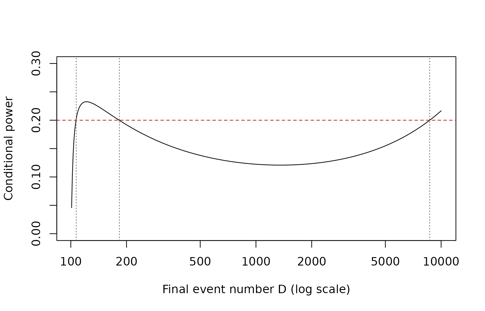

Worked TrialSimulator example

We now simulate one two-arm trial with an event-driven endpoint. A calendar milestone provides the locked interim data used by both methods.

pfs_pbo <- endpoint(name = 'pfs', type = 'tte', generator = rexp,
                    rate = log(2) / 10)
pbo <- arm(name = 'pbo')
pbo$add_endpoints(pfs_pbo)

pfs_trt <- endpoint(name = 'pfs', type = 'tte', generator = rexp,
                    rate = log(2) / 14)
trt <- arm(name = 'trt')
trt$add_endpoints(pfs_trt)

accrual_rate <- data.frame(end_time = Inf, piecewise_rate = 30)
trial <- trial(name = 'cp-example', n_patients = 400, duration = 40,
               seed = 31416, enroller = StaggeredRecruiter,
               accrual_rate = accrual_rate, silent = TRUE)
trial$add_arms(sample_ratio = c(1, 1), pbo, trt)

interim <- milestone(name = 'interim', when = calendarTime(time = 15))
final <- milestone(name = 'final', when = calendarTime(time = 40))

listener <- listener(silent = TRUE)
listener$add_milestones(interim, final)

controller <- controller(trial, listener)
controller$run(n = 1, silent = TRUE, plot_event = FALSE)

The next subsections deliberately analyze this completed replicate directly, outside a milestone action function. This is diagnostic code: it makes the inputs and outputs easy to compare while demonstrating effect assumptions, alternative directions, caps, and return values one feature at a time. It is not the recommended structure for a simulation study. After these focused examples, see the implementation of promising_zone_action() and the complete event-driven simulation program for the recommended TrialSimulator structure.

When 'interim' is supplied as milestone, each method retrieves the data locked at that milestone and calls fitLogrank() internally. The explicit fit below reproduces that internal step so that the resulting interim logrank statistic z and event count info—denoted by $z$ and $d$ in the formulas, and returned as z and d by the methods—are visible. interim_fit is not an input to either method and need not be fitted beforehand. Likewise, the direct method calls that follow are intentional teaching devices rather than actions that can adapt this already completed trial.

interim_fit <- fitLogrank(
  Surv(pfs, pfs_event) ~ arm,
  placebo = 'pbo', data = trial$get_locked_data('interim'),
  alternative = 'less', tidy = FALSE
)
interim_fit[, c('arm', 'placebo', 'z', 'info')]
#>   arm placebo         z info
#> 1 trt     pbo -1.092148  145

Conditional power under different assumptions

Suppose the planned final analysis has 300 events and its one-sided final boundary corresponds to nominal alpha = 0.022.

planned_D <- 300
final_alpha <- 0.022

cp_at <- function(effect){
  trial$conditionalPower(
    'interim', Surv(pfs, pfs_event) ~ arm,
    placebo = 'pbo', alternative = 'less',
    alpha = final_alpha, D = planned_D, effect = effect
  )$cp
}

data.frame(
  assumption = c('interim trend', 'null future drift', 'hazard ratio 0.75'),
  conditional_power = c(cp_at('trend'), cp_at('null'), cp_at(0.75))
)
#>          assumption conditional_power
#> 1     interim trend        0.26877360
#> 2 null future drift        0.04043096
#> 3 hazard ratio 0.75        0.51798610

The difference between the trend and specified-effect calculations is not a software discrepancy: they answer different conditional questions. A robust design should examine assumptions chosen before looking at the interim result.

The direction transformation can also be checked directly by swapping the reference arm. The treatment-vs-placebo hazard ratio 0.75 becomes the placebo-vs-treatment hazard ratio $1/0.75$, and "less" becomes "greater".

cp_less <- trial$conditionalPower(
  'interim', Surv(pfs, pfs_event) ~ arm,
  placebo = 'pbo', alternative = 'less',
  alpha = final_alpha, D = planned_D, effect = 0.75
)

cp_greater <- trial$conditionalPower(
  'interim', Surv(pfs, pfs_event) ~ arm,
  placebo = 'trt', alternative = 'greater',
  alpha = final_alpha, D = planned_D, effect = 1 / 0.75
)

data.frame(
  formulation = c('trt vs pbo, less', 'pbo vs trt, greater'),
  z = c(cp_less$z, cp_greater$z),
  conditional_power = c(cp_less$cp, cp_greater$cp)
)
#>           formulation         z conditional_power
#> 1    trt vs pbo, less -1.092148         0.5179861
#> 2 pbo vs trt, greater  1.092148         0.5179861

Event-number reassessment and the cap

Under the assumed hazard ratio 0.75, request 90% conditional power. Comparing two caps illustrates both possible values of target_reached; the smaller cap remains recorded in D_cap, while D and achieved_cp are NA because no solution exists through that cap.

reassess_500 <- trial$eventNumberReestimationFromConditionalPower(
  'interim', Surv(pfs, pfs_event) ~ arm,
  placebo = 'pbo', alternative = 'less',
  alpha = final_alpha, target_cp = 0.9,
  effect = 0.75, D_cap = 500
)

reassess_600 <- trial$eventNumberReestimationFromConditionalPower(
  'interim', Surv(pfs, pfs_event) ~ arm,
  placebo = 'pbo', alternative = 'less',
  alpha = final_alpha, target_cp = 0.9,
  effect = 0.75, D_cap = 600
)

rbind(cap_500 = reassess_500, cap_600 = reassess_600)[,
  c('d', 'D', 'D_cap', 'target_cp', 'achieved_cp', 'target_reached')]
#>           d   D D_cap target_cp achieved_cp target_reached
#> cap_500 145  NA   500       0.9          NA          FALSE
#> cap_600 145 574   600       0.9   0.9005152           TRUE

Omitting D_cap, or passing NULL, requests the unbounded answer and is equivalent here to the solution under cap 600.

trial$eventNumberReestimationFromConditionalPower(
  'interim', Surv(pfs, pfs_event) ~ arm,
  placebo = 'pbo', alternative = 'less',
  alpha = final_alpha, target_cp = 0.9, effect = 0.75
)[, c('d', 'D', 'D_cap', 'achieved_cp', 'target_reached')]
#>     d   D D_cap achieved_cp target_reached
#> 1 145 574   Inf   0.9005152           TRUE

A promising-zone policy

A common design pattern classifies conditional power at the originally planned final event number into zones. The following thresholds are purely illustrative:

• unfavorable: $CP(D_{\text{planned}})<0.30$;
• promising: $0.30\leq CP(D_{\text{planned}})<0.90$;
• favorable: $CP(D_{\text{planned}})\geq0.90$.

For the specified hazard ratio 0.75, the worked example lies in the promising zone.

lower_cp <- 0.30
target_cp <- 0.90
cp_planned <- cp_at(0.75)

zone <- if(cp_planned < lower_cp){
  'unfavorable'
}else if(cp_planned < target_cp){
  'promising'
}else{
  'favorable'
}

data.frame(planned_D, cp_planned, zone,
           reassessed_D = reassess_600$D,
           target_reached = reassess_600$target_reached)
#>   planned_D cp_planned      zone reassessed_D target_reached
#> 1       300  0.5179861 promising          574           TRUE

One possible pre-specified policy is to retain the original design in the unfavorable and favorable zones, and increase the event target in the promising zone subject to a cap. A different design could stop for futility in the unfavorable zone. These choices are properties of the trial design, not of the calculator.

Implementing the policy in an action function

The following function implements the increase-only rule at an interim milestone. The final milestone must already be registered and must not yet have triggered. The complete program near the end of this vignette registers this action and executes the simulation.

promising_zone_action <- function(trial){
  ## Pre-specified design parameters. The promising zone is defined using
  ## conditional power at the originally planned final analysis.
  planned_D <- 300
  lower_cp <- 0.30
  target_cp <- 0.90
  D_cap <- 600

  ## conditionalPower() obtains the data locked at the interim milestone
  ## and fits the treatment-vs-placebo logrank comparison internally.
  cp <- trial$conditionalPower(
    'interim', Surv(pfs, pfs_event) ~ arm,
    placebo = 'pbo', alternative = 'less',
    alpha = 0.022, D = planned_D, effect = 0.75
  )$cp

  if(cp < lower_cp){
    zone <- 'unfavorable'
    decision <- 'unfavorable: retain planned event number'
    selected_D <- planned_D
  }else if(cp < target_cp){
    zone <- 'promising'

    ## Only a promising result invokes event-number reassessment. The solver
    ## searches for the earliest solution after the observed interim events.
    reassessment <- trial$eventNumberReestimationFromConditionalPower(
      'interim', Surv(pfs, pfs_event) ~ arm,
      placebo = 'pbo', alternative = 'less',
      alpha = 0.022, target_cp = target_cp,
      effect = 0.75, D_cap = D_cap
    )

    ## This policy permits increases only. Use the exact solution when it is
    ## above planned_D; otherwise use the pre-specified cap as the fallback.
    if(reassessment$target_reached && reassessment$D > planned_D){
      selected_D <- reassessment$D
      decision <- 'promising: reassess to target conditional power'
    }else{
      selected_D <- reassessment$D_cap
      decision <- if(reassessment$target_reached){
        'promising: use cap because the earliest solution is not an increase'
      }else{
        'promising: use cap because no solution was found through the cap'
      }
    }

  }else{
    zone <- 'favorable'
    decision <- 'favorable: retain the planned design'
    selected_D <- planned_D
  }

  ## update_milestone() must be called from a milestone action. It queues a
  ## replacement for the registered, not-yet-triggered final milestone. The
  ## new event target takes effect after this action returns and applies only
  ## to the current replicate; the original trigger is restored before the
  ## next replicate. No update is needed when planned_D is retained.
  if(selected_D > planned_D){
    trial$update_milestone(
      'final',
      when = eventNumber(endpoint = 'pfs', n = selected_D,
                         arms = c('pbo', 'trt'))
    )
  }

  ## Re-evaluate conditional power at the event number that will actually be
  ## used as the final target, including a cap selected as a fallback.
  selected_cp <- trial$conditionalPower(
    'interim', Surv(pfs, pfs_event) ~ arm,
    placebo = 'pbo', alternative = 'less',
    alpha = 0.022, D = selected_D, effect = 0.75
  )$cp

  ## Values saved in an action function become simulation-output columns.
  trial$save(zone, 'promising_zone')
  trial$save(cp, 'conditional_power_at_planned_D')
  trial$save(selected_D, 'selected_final_event_number')
  trial$save(selected_cp, 'conditional_power_at_final_D')
  trial$save(selected_cp >= target_cp, 'target_reached_at_selected_D')
  trial$save(decision, 'promising_zone_decision')
}

The queued update replaces the complete trigger condition of the registered final milestone; it does not trigger the final analysis immediately. Here, eventNumber(..., arms = c('pbo', 'trt')) makes the new condition count PFS events on the two comparison arms. After the action returns, the listener applies this condition before checking subsequent milestones. The automatic reset between replicates is important: each simulated trial starts from the same as-designed 300-event final milestone rather than inheriting the previous replicate’s reassessment.

Many promising-zone designs permit an increase but not a decrease from the originally planned event number. The reassessment method itself searches from $d+1$, not from planned_D. Therefore, an increase-only policy must verify that the returned D is at least planned_D. In a nonmonotone case, simply replacing a smaller result by planned_D is not guaranteed to preserve the target conditional power; the admissible search domain and action should be pre-specified explicitly. The action above uses D_cap as its pre-specified increase-only fallback and separately records whether conditional power at that selected event number reaches the target.

Assumptions and design checks

Before using these calculations in a design, check the following.

1. The final statistic and boundary must match the canonical calculation. The allocation ratio should remain constant, and the compared treatment and placebo arms should be concurrently enrolled.
2. alpha must represent the nominal final boundary, not an arbitrary overall alpha or final-stage alpha increment.
3. The effect assumption should be pre-specified. Report sensitivity to the interim trend and clinically relevant fixed hazard ratios when useful.
4. D_cap should reflect a feasible event budget. Inspect target_reached; when it is FALSE, both D and achieved_cp are NA.
5. The operational rule must distinguish a final boundary from a formal interim stopping boundary.
6. Simulate the entire adaptive design under the null and relevant alternatives. Unblinded sample-size or event-number changes can inflate type I error unless the testing procedure or the restricted adaptation rule has been justified.

TrialSimulator computes the stated conditional quantities but cannot verify that a data-dependent adaptation is valid for a particular confirmatory trial. If adaptation changes the final statistic, information weights, allocation, or critical boundary, use an appropriate adaptive or combination-test analysis rather than treating the original final test as unchanged.

A complete promising-zone simulation

The earlier trial object was deliberately small and was used only to inspect a single locked dataset. We now redefine it with enough patients and follow-up to make every event target through D_cap = 600 feasible. The interim and final analyses are event driven. The interim action is promising_zone_action() defined above; the final action performs the planned logrank test and saves the result.

promising_zone_final_action <- function(trial){
  fit <- fitLogrank(
    Surv(pfs, pfs_event) ~ arm,
    placebo = 'pbo', data = trial$get_locked_data('final'),
    alternative = 'less', tidy = FALSE
  )

  trial$save(fit$info, 'observed_final_event_number')
  trial$save(fit$z, 'final_z')
  trial$save(fit$p, 'final_p')
  trial$save(fit$p <= 0.022, 'reject_final')
}

The following is a complete simulation program: arms, trial, milestone actions, listener, and controller are all connected before execution. The initial final milestone requests 300 events. When the interim action selects a larger target, update_milestone() replaces that trigger for the current replicate only; the listener restores the original 300-event trigger before the next replicate.

pfs_pbo <- endpoint(name = 'pfs', type = 'tte', generator = rexp,
                    rate = log(2) / 10)
pbo <- arm(name = 'pbo')
pbo$add_endpoints(pfs_pbo)

pfs_trt <- endpoint(name = 'pfs', type = 'tte', generator = rexp,
                    rate = 0.75 * log(2) / 10)
trt <- arm(name = 'trt')
trt$add_endpoints(pfs_trt)

accrual_rate <- data.frame(end_time = Inf, piecewise_rate = 30)
trial <- trial(
  name = 'promising-zone', n_patients = 700, duration = 120,
  seed = 20260831, enroller = StaggeredRecruiter,
  accrual_rate = accrual_rate, silent = TRUE
)
trial$add_arms(sample_ratio = c(1, 1), pbo, trt)

interim <- milestone(
  name = 'interim', action = promising_zone_action,
  when = eventNumber(endpoint = 'pfs', n = 150,
                     arms = c('pbo', 'trt'))
)
final <- milestone(
  name = 'final', action = promising_zone_final_action,
  when = eventNumber(endpoint = 'pfs', n = 300,
                     arms = c('pbo', 'trt'))
)

listener <- listener(silent = TRUE)
listener$add_milestones(interim, final)

controller <- controller(trial, listener)
controller$run(n = 1, silent = TRUE, plot_event = FALSE)

The saved columns show the complete path from the interim zone and selected event target to the final test for this replicate.

Decision path and final analysis for one replicate

Zone	CP at planned D	Selected final D	CP at final D	Target reached	Observed final D	Final p-value	Reject
promising	0.516	572	0.9	TRUE	572	0.00159	TRUE

For operating characteristics, increase n after resetting the controller. The following code produces the 1000-replicate output summarized below.

controller$reset()
controller$run(n = 1000, silent = TRUE, plot_event = FALSE)
conditional_power_output <- controller$get_output()

Here are the first five replicates, restricted to the main decision and final analysis columns.

Decision and final-analysis results for the first five replicates

Zone	CP at planned D	Selected final D	CP at final D	Target reached	Observed final D	Final p-value	Reject
promising	0.516	572	0.900	TRUE	572	0.00159	TRUE
favorable	1.000	300	1.000	TRUE	300	< 0.001	TRUE
promising	0.384	600	0.882	FALSE	600	0.00133	TRUE
favorable	0.929	300	0.929	TRUE	300	< 0.001	TRUE
promising	0.340	600	0.867	FALSE	600	0.00662	TRUE

The zone frequencies and mean selected event number summarize how often the rule adapts the final milestone when both the data-generating and conditional-power hazard ratios are 0.75.

Promising-zone frequency and selected event number

Zone	Replicates	Percent (%)	Mean selected D
unfavorable	125	12.5	300.0
promising	627	62.7	516.9
favorable	248	24.8	300.0

Finally, the overall summary connects adaptation frequency, attainment of the conditional-power target at the selected event number, and the final testing result. These values describe this illustrative data-generating scenario; they do not establish type I error control for the adaptation rule.

Operating characteristics of the promising-zone design

Operating characteristic	Percent (%)
final event target increased	62.7
target CP reached at selected D	77.5
final null hypothesis rejected	82.9

Multiple treatment arms

Both methods support several treatment-placebo comparisons. D, alpha, target_cp, and a non-scalar finite D_cap are named by treatment arm. Names, not vector positions, determine matching.

The setup of the following three-arm toy trial is executed but not printed in the rendered vignette. Its complete code remains in the Rmd source. This section is intentionally limited to demonstrating the multi-comparison output format and name-based argument matching; the detailed design examples remain focused on a single treatment-placebo comparison. To isolate the example, it is the vignette’s last executable section, and its construction occurs inside local(): only the trial object needed by the two displayed calls leaves the setup scope.

trial$conditionalPower(
  'interim', Surv(pfs, pfs_event) ~ arm,
  placebo = 'pbo', alternative = 'less',
  D = c(low = 350, high = 400),
  alpha = c(high = 0.01, low = 0.015),
  effect = 0.75
)
#>    arm placebo         z   d   D info_fraction alpha effect        cp
#> 1  low     pbo -1.918441 173 350     0.4942857 0.015   0.75 0.7759951
#> 2 high     pbo -3.208487 161 400     0.4025000 0.010   0.75 0.9676651

trial$eventNumberReestimationFromConditionalPower(
  'interim', Surv(pfs, pfs_event) ~ arm,
  placebo = 'pbo', alternative = 'less',
  alpha = c(low = 0.015, high = 0.01),
  target_cp = c(high = 0.90, low = 0.85),
  effect = 'trend',
  D_cap = c(low = 600, high = 700)
)
#>    arm placebo         z   d   D D_cap alpha effect target_cp achieved_cp
#> 1  low     pbo -1.918441 173 412   600 0.015  trend      0.85   0.8503304
#> 2 high     pbo -3.208487 161 162   700 0.010  trend      0.90   1.0000000
#>   target_reached
#> 1           TRUE
#> 2           TRUE

Event counts are pair-specific: each d and D counts events on placebo plus one treatment arm. With a shared placebo, event counts across comparisons need not sum to a trial-wide total.

References

• Chen, Y. H. J., DeMets, D. L., and Lan, K. K. G. (2004). Increasing the sample size when the unblinded interim result is promising. Statistics in Medicine, 23, 1023–1038. https://doi.org/10.1002/sim.1688
• Cui, L., Hung, H. M. J., and Wang, S.-J. (1999). Modification of sample size in group sequential clinical trials. Biometrics, 55, 853–857. https://doi.org/10.1111/j.0006-341X.1999.00853.x
• Mehta, C. R., and Pocock, S. J. (2011). Adaptive increase in sample size when interim results are promising: a practical guide with examples. Statistics in Medicine, 30, 3267–3284. https://doi.org/10.1002/sim.4102